Questions.
1. What type of motion - uniform or non-uniform - does rectilinear uniformly accelerated motion belong to?
Rectilinear uniformly accelerated motion refers to non-uniform motion, because it occurs at a variable (time-varying in magnitude and direction) speed.
2. What is meant by instantaneous speed uneven movement?
The instantaneous speed of uneven movement is understood as the speed at a specific point of the trajectory in this moment time.
3. What is called acceleration uniformly accelerated motion?
4. What is uniformly accelerated motion?
Motion with constant acceleration is called uniformly accelerated motion.
5. What does the magnitude of the acceleration vector show?
6. What is the unit of acceleration?
In SI, the unit of acceleration is taken to be the acceleration of such uniformly accelerated motion, in which in 1 second the speed of the body changes by 1 m/s, i.e. 1 m/s 2 (meter per second squared, or in other words 1 meter per second per second).
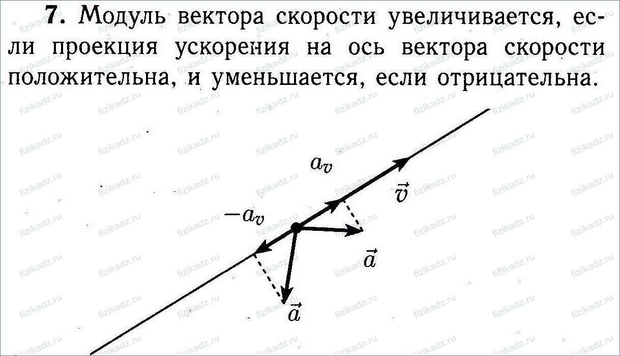
7. Under what condition does the magnitude of the velocity vector of a moving body increase? is it decreasing?
Exercises.
1. Over the same period of time, the magnitude of the velocity vector of the first car changed from v 1 to v´, and the second - from v 2 to v´ (velocities are shown on the same scale in Figure 9). Which car was moving at the indicated interval with greater acceleration? Which one increased in speed faster?
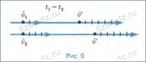
The figure shows that the speed of the first car increased faster than the second, and therefore it had greater acceleration.
2. The plane, accelerating before takeoff, moved uniformly accelerated for a certain period of time. What was the acceleration of the plane if in 30 s its speed increased from 10 to 55 m/s?
3. With what acceleration did the train move on a certain section of the track if its speed increased by 6 m/s in 12 s?
In addition to the total acceleration determined by (2.6), there are two more accelerations. It is easy to verify this by replacing the velocity vector with the product:
where is the unit vector directed along the velocity. Then the acceleration vector, as a derivative of the product of two functions, will appear as the sum of two vectors:
each of which is one of the components of the acceleration vector.
Let's call the first of these vectors tangential acceleration, since it is directed tangentially to the trajectory:
Obviously, tangential acceleration characterizes speed of change of speed module(vector length). The magnitude of the vector, or more precisely, its projection onto the direction of velocity, is defined as the derivative of the velocity modulus with respect to time:
The last equation shows that a t may have a sign: it will be negative if the speed decreases, because in this case d u – the increment of the speed module is negative. Movement with decreasing speed is called slow. It is obvious that during slow motion the tangential acceleration vector is directed opposite to the velocity vector.
The second vector in sum (2.8) is called normal acceleration. This vector is related to the rate of change directions speed Magnitude and direction of the normal acceleration vector
we will find from the following considerations.
First of all, from (2.8) it follows that the total acceleration will be equal to normal if the tangential acceleration is equal to zero. If we add to this the definition of total acceleration (2.6), we get:
The index entered into the equation n, which was not there before, means that the velocity increment is taken for the special case when the tangential acceleration is zero, that is, the length of the velocity vector does not change. Under this condition, Fig. will also change. 2.5, where the vector is directed at an angle to the trajectory, varying depending on the ratio of the lengths of the vectors.
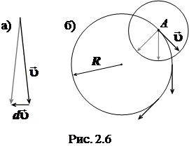 In Fig. Figure 2.6a shows two velocity vectors of equal length. In this case, the vector of their change is directed at an angle close to a straight line. The same thing is observed when constructing the drawing in Fig. 2.6b, where the point moves along a circle of radius R
, without changing the value of its speed. The vectors are depicted at three points, and to find the increment of the velocity vector, the beginnings of the vectors are moved to the point A.
In Fig. Figure 2.6a shows two velocity vectors of equal length. In this case, the vector of their change is directed at an angle close to a straight line. The same thing is observed when constructing the drawing in Fig. 2.6b, where the point moves along a circle of radius R
, without changing the value of its speed. The vectors are depicted at three points, and to find the increment of the velocity vector, the beginnings of the vectors are moved to the point A.
If we sequentially depict the velocity vectors at all points of the circle, and then, to find the vectors of their differences, move their origins to the point A, we get a second circle made up of vectors .
The radius of the circle will be the modulus u velocity vector. The length of this new circle is 2 pu will be the sum of the moduli of individual vectors during the time until the point makes a full revolution along its path 2 p R . This time will be equal to the ratio of the path traveled by the point to the speed of its movement:
If, following (2.12), the change in speed is divided by the time during which it occurred, we obtain the modulus of normal acceleration:
The direction of normal acceleration coincides with the vector, and the last vector is always perpendicular to the speed, since it is an element of a circle in which the speed is the radius (see Fig. 2.6).
The velocity is always directed tangentially to the trajectory, which means the normal acceleration is directed radially to the center of its curvature. That's why it is also called centripetal.
So, having defined the third kinematic characteristic motion of a material point - total acceleration according to (2.6) - we came to the conclusion that there are two more types of acceleration - tangential and normal, the modules of which are found according to (2.10) and (2.14), respectively. In Fig. Figure 2.7 shows the vectors of these accelerations at one point of the curvilinear trajectory. Naturally, they are perpendicular to each other. According to (2.8) their geometric sum should give full acceleration, which, as in Fig. 2.4, directed at an angle to the trajectory inside its curvature:
Full acceleration module:
All three accelerations characterize uneven movement along a curve. At uniform motion along any trajectory a t = 0, and when moving in a straight line, the normal acceleration vanishes.
IN general case When a point moves, its speed changes over time. Let us introduce a quantity characterizing this change.
Let the position of the point be determined by the radius vector. Each moment t will correspond to a certain velocity vector applied to the point and directed tangentially to the hodograph of the radius vector (Fig. 21, a). All velocity vectors applied to point M at different times are depicted in Fig. 21, b. The geometric location of the ends of the velocity vectors will be the hodograph of the velocity vector.
Let at the moment of time t the position of the point M be determined by the radius vector and its speed will be and at the moment of time the position of the point will be determined by the radius vector and its speed will be (Fig. 21, a and b). Vector difference
![]()
is depicted as a chord subtending the arc of the velocity hodograph (Fig. 21, b).
The vector defined by the equality:
![]()
is called the acceleration vector (or simply acceleration) of point M at time . Since the velocity vector is the first derivative with respect to time of the radius of the vector, we can write:
![]()
i.e., the acceleration vector is equal to the first derivative of the velocity vector and the second derivative of the vector radius with respect to time.
Note that the differentiation rule is applied to vectors that are always applied to points M and O, respectively. The vector characterizing the movement of point M is applied to this point.
Just as the velocity vector is directed tangent to the hodograph of the radius vector, the acceleration vector is directed tangent to the hodograph of the velocity vector; its location relative to the trajectory requires special research. Since the acceleration is completely determined by the type of function that does not depend on the choice of a fixed coordinate system, then the acceleration is vector quantity, which characterizes the movement itself and does not depend on the choice of a fixed coordinate system.
Orthogonal projections of the acceleration vector
Denoting the acceleration projections on the x, y, z axes, we write