Linear equations. Solution, examples

Etc., it is logical to get acquainted with equations of other types. Next in line are linear equations, the targeted study of which begins in algebra lessons in the 7th grade.

It is clear that first we need to explain what a linear equation is, give a definition of a linear equation, its coefficients, and show its general form. Then you can figure out how many solutions a linear equation has depending on the values ​​of the coefficients, and how the roots are found. This will allow you to move on to solving examples, and thereby consolidate the learned theory. In this article we will do this: we will dwell in detail on all the theoretical and practical points relating to linear equations and their solutions.

Let’s say right away that here we will consider only linear equations with one variable, and in a separate article we will study the principles of solution linear equations with two variables.

Page navigation.

What is a linear equation?

The definition of a linear equation is given by the way it is written. Moreover, in different mathematics and algebra textbooks, the formulations of the definitions of linear equations have some differences that do not affect the essence of the issue.

For example, in the algebra textbook for grade 7 by Yu. N. Makarychev et al., a linear equation is defined as follows:

Definition.

Equation of the form a x=b, where x is a variable, a and b are some numbers, is called linear equation with one variable.

Let us give examples of linear equations that meet the stated definition. For example, 5 x = 10 is a linear equation with one variable x, here the coefficient a is 5, and the number b is 10. Another example: −2.3·y=0 is also a linear equation, but with a variable y, in which a=−2.3 and b=0. And in linear equations x=−2 and −x=3.33 a are not present explicitly and are equal to 1 and −1, respectively, while in the first equation b=−2, and in the second - b=3.33.

And a year earlier, in the textbook of mathematics by N. Ya. Vilenkin, linear equations with one unknown, in addition to equations of the form a x = b, also considered equations that can be brought to this form by transferring terms from one part of the equation to another with the opposite sign, as well as by reducing similar terms. According to this definition, equations of the form 5 x = 2 x + 6, etc. also linear.

In turn, in the algebra textbook for grade 7 by A. G. Mordkovich the following definition is given:

Definition.

Linear equation with one variable x is an equation of the form a·x+b=0, where a and b are some numbers called coefficients of the linear equation.

For example, linear equations of this type are 2 x−12=0, here the coefficient a is 2, and b is equal to −12, and 0.2 y+4.6=0 with coefficients a=0.2 and b =4.6. But at the same time, there are examples of linear equations that have the form not a·x+b=0, but a·x=b, for example, 3·x=12.

Let us, so that we do not have any discrepancies in the future, by a linear equation with one variable x and coefficients a and b we mean an equation of the form a x + b = 0. This type of linear equation seems to be the most justified, since linear equations are algebraic equations first degree. And all the other equations indicated above, as well as equations that, using equivalent transformations, are reduced to the form a x + b = 0, we will call equations that reduce to linear equations. With this approach, the equation 2 x+6=0 is a linear equation, and 2 x=−6, 4+25 y=6+24 y, 4 (x+5)=12, etc. - These are equations that reduce to linear ones.

How to solve linear equations?

Now it’s time to figure out how linear equations a·x+b=0 are solved. In other words, it's time to find out whether a linear equation has roots, and if so, how many of them and how to find them.

The presence of roots of a linear equation depends on the values ​​of the coefficients a and b. In this case, the linear equation a x+b=0 has

• the only root for a≠0,
• has no roots for a=0 and b≠0,
• has infinitely many roots for a=0 and b=0, in which case any number is a root of a linear equation.

Let us explain how these results were obtained.

We know that to solve equations we can move from the original equation to equivalent equations, that is, to equations with the same roots or, like the original one, without roots. To do this, you can use the following equivalent transformations:

• transferring a term from one side of the equation to another with the opposite sign,
• as well as multiplying or dividing both sides of an equation by the same non-zero number.

So, in a linear equation with one variable of the form a·x+b=0, we can move the term b from the left side to the right side with the opposite sign. In this case, the equation will take the form a·x=−b.

And then it begs the question of dividing both sides of the equation by the number a. But there is one thing: the number a can be equal to zero, in which case such division is impossible. To deal with this problem, we will first assume that the number a is non-zero, and we will consider the case of a being equal to zero separately a little later.

So, when a is not equal to zero, then we can divide both sides of the equation a·x=−b by a, after which it will be transformed to the form x=(−b):a, this result can be written using the fractional slash as.

Thus, for a≠0, the linear equation a·x+b=0 is equivalent to the equation, from which its root is visible.

It is easy to show that this root is unique, that is, the linear equation has no other roots. This allows you to do the opposite method.

Let's denote the root as x 1. Let us assume that there is another root of the linear equation, which we denote as x 2, and x 2 ≠x 1, which, due to determining equal numbers through difference is equivalent to the condition x 1 −x 2 ≠0. Since x 1 and x 2 are roots of the linear equation a·x+b=0, then the numerical equalities a·x 1 +b=0 and a·x 2 +b=0 hold. We can subtract the corresponding parts of these equalities, which the properties of numerical equalities allow us to do, we have a·x 1 +b−(a·x 2 +b)=0−0, from which a·(x 1 −x 2)+( b−b)=0 and then a·(x 1 −x 2)=0 . But this equality is impossible, since both a≠0 and x 1 − x 2 ≠0. So we came to a contradiction, which proves the uniqueness of the root of the linear equation a·x+b=0 for a≠0.

This is how we solved the linear equation a·x+b=0 for a≠0. The first result given at the beginning of this paragraph is justified. There are two more left that meet the condition a=0.

When a=0, the linear equation a·x+b=0 takes the form 0·x+b=0. From this equation and the property of multiplying numbers by zero it follows that no matter what number we take as x, when it is substituted into the equation 0 x + b=0, the numerical equality b=0 will be obtained. This equality is true when b=0, and in other cases when b≠0 this equality is false.

Consequently, with a=0 and b=0, any number is the root of the linear equation a·x+b=0, since under these conditions, substituting any number for x gives the correct numerical equality 0=0. And when a=0 and b≠0, the linear equation a·x+b=0 has no roots, since under these conditions, substituting any number instead of x leads to the incorrect numerical equality b=0.

The given justifications allow us to formulate a sequence of actions that allows us to solve any linear equation. So, algorithm for solving linear equation is:

• First, by writing the linear equation, we find the values ​​of the coefficients a and b.
• If a=0 and b=0, then this equation has infinitely many roots, namely, any number is a root of this linear equation.
• If a is nonzero, then
• the coefficient b is transferred to the right side with the opposite sign, and the linear equation is transformed to the form a·x=−b,
• after which both sides of the resulting equation are divided by a nonzero number a, which gives the desired root of the original linear equation.

The written algorithm is a comprehensive answer to the question of how to solve linear equations.

In conclusion of this point, it is worth saying that a similar algorithm is used to solve equations of the form a·x=b. Its difference is that when a≠0, both sides of the equation are immediately divided by this number; here b is already in the required part of the equation and there is no need to transfer it.

To solve equations of the form a x = b, the following algorithm is used:

• If a=0 and b=0, then the equation has infinitely many roots, which are any numbers.
• If a=0 and b≠0, then the original equation has no roots.
• If a is non-zero, then both sides of the equation are divided by a non-zero number a, from which the only root of the equation is found, equal to b/a.

Examples of solving linear equations

Let's move on to practice. Let's look at how the algorithm for solving linear equations is used. Let us present solutions to typical examples corresponding to different values ​​of the coefficients of linear equations.

Example.

Solve the linear equation 0·x−0=0.

Solution.

In this linear equation, a=0 and b=−0 , which is the same as b=0 . Therefore, this equation has infinitely many roots; any number is a root of this equation.

Answer:

x – any number.

Example.

Does the linear equation 0 x + 2.7 = 0 have solutions?

Solution.

In this case, coefficient a is equal to zero, and coefficient b of this linear equation is equal to 2.7, that is, different from zero. Therefore, a linear equation has no roots.

A linear equation is an algebraic equation whose total degree of polynomials is equal to one. Solving linear equations is part of the school curriculum, and not the most difficult one. However, some still have difficulty completing this topic. We hope that after reading this material, all difficulties for you will remain in the past. So, let's figure it out. how to solve linear equations.

General form

The linear equation is represented as:

• ax + b = 0, where a and b are any numbers.

Although a and b can be any number, their values ​​affect the number of solutions to the equation. There are several special cases of solution:

• If a=b=0, the equation has an infinite number of solutions;
• If a=0, b≠0, the equation has no solution;
• If a≠0, b=0, the equation has a solution: x = 0.

In the event that both numbers have non-zero values, the equation must be solved to derive the final expression for the variable.

How to decide?

Solving a linear equation means finding what the variable is equal to. How to do this? Yes, it’s very simple - using simple algebraic operations and following the rules of transfer. If the equation appears in front of you in general form, you are in luck; all you need to do is:

1. Move b to the right side of the equation, not forgetting to change the sign (transfer rule!), thus, from an expression of the form ax + b = 0, an expression of the form should be obtained: ax = -b.
2. Apply the rule: to find one of the factors (x - in our case), you need to divide the product (-b in our case) by another factor (a - in our case). Thus, you should get an expression of the form: x = -b/a.

That's it - a solution has been found!

Now let's look at a specific example:

1. 2x + 4 = 0 - move b, equal to 4 in this case, to the right side
2. 2x = -4 - divide b by a (don’t forget about the minus sign)
3. x = -4/2 = -2

That's all! Our solution: x = -2.

As you can see, the solution to a linear equation with one variable is quite simple to find, but everything is so simple if we are lucky enough to come across the equation in its general form. In most cases, before solving an equation in the two steps described above, you still need to bring the existing expression to a general form. However, this is also not an extremely difficult task. Let's look at some special cases using examples.

Solving special cases

First, let's look at the cases that we described at the beginning of the article and explain what it means to have an infinite number of solutions and no solution.

• If a=b=0, the equation will look like: 0x + 0 = 0. Performing the first step, we get: 0x = 0. What does this nonsense mean, you exclaim! After all, no matter what number you multiply by zero, you always get zero! Right! That's why they say that the equation has an infinite number of solutions - no matter what number you take, the equality will be true, 0x = 0 or 0=0.
• If a=0, b≠0, the equation will look like: 0x + 3 = 0. Perform the first step, we get 0x = -3. Nonsense again! It is obvious that this equality will never be true! That's why they say that the equation has no solutions.
• If a≠0, b=0, the equation will look like: 3x + 0 = 0. Performing the first step, we get: 3x = 0. What is the solution? It's easy, x = 0.

Lost in translation

The described special cases are not all that linear equations can surprise us with. Sometimes the equation is difficult to identify at first glance. Let's look at an example:

• 12x - 14 = 2x + 6

Is this a linear equation? What about the zero on the right side? Let's not rush to conclusions, let's act - let's move all the components of our equation to the left. We get:

• 12x - 2x - 14 - 6 = 0

Now subtract like from like, we get:

• 10x - 20 = 0

Learned? The most linear equation ever! The solution to which is: x = 20/10 = 2.

What if we have this example:

• 12((x + 2)/3) + x) = 12 (1 - 3x/4)

Yes, this is also a linear equation, only more transformations need to be carried out. First, let's open the brackets:

1. (12(x+2)/3) + 12x = 12 - 36x/4
2. 4(x+2) + 12x = 12 - 36x/4
3. 4x + 8 + 12x = 12 - 9x - now we carry out the transfer:
4. 25x - 4 = 0 - it remains to find a solution using the already known scheme:
5. 25x = 4,
6. x = 4/25 = 0.16

As you can see, everything can be solved, the main thing is not to worry, but to act. Remember, if your equation contains only variables of the first degree and numbers, you have a linear equation, which, no matter how it looks initially, can be reduced to a general form and solved. We hope everything works out for you! Good luck!

When solving linear equations, we strive to find the root, that is, the value for the variable that will turn the equation into a correct equality.

To find the root of the equation you need equivalent transformations bring the equation given to us to the form

\(x=[number]\)

This number will be the root.

That is, we transform the equation, making it simpler with each step, until we reduce it to a completely primitive equation “x = number”, where the root is obvious. The most frequently used transformations when solving linear equations are the following:

For example: add \(5\) to both sides of the equation \(6x-5=1\)

\(6x-5=1\) \(|+5\)
\(6x-5+5=1+5\)
\(6x=6\)

Please note that we could get the same result faster by simply writing the five on the other side of the equation and changing its sign. Actually, this is exactly how the school “transfer through equals with a change of sign to the opposite” is done.

2. Multiplying or dividing both sides of an equation by the same number or expression.

For example: divide the equation \(-2x=8\) by minus two

\(-2x=8\) \(|:(-2)\)
\(x=-4\)

Typically this step is performed at the very end, when the equation has already been reduced to the form \(ax=b\), and we divide by \(a\) to remove it from the left.

3. Using the properties and laws of mathematics: opening parentheses, bringing similar terms, reducing fractions, etc.

Add \(2x\) left and right

Subtract \(24\) from both sides of the equation

We present similar terms again

Now we divide the equation by \(-3\), thereby removing the front X on the left side.

Answer : \(7\)

The answer has been found. However, let's check it out. If seven is really a root, then when substituting it instead of X in the original equation, the correct equality should be obtained - the same numbers on the left and on the right. Let's try.

Examination:
\(6(4-7)+7=3-2\cdot7\)
\(6\cdot(-3)+7=3-14\)
\(-18+7=-11\)
\(-11=-11\)

It worked out. This means that seven is indeed the root of the original linear equation.

Don’t be lazy to check the answers you found by substitution, especially if you are solving an equation on a test or exam.

The question remains - how to determine what to do with the equation at the next step? How exactly to convert it? Divide by something? Or subtract? And what exactly should I subtract? Divide by what?

The answer is simple:

Your goal is to bring the equation to the form \(x=[number]\), that is, on the left is x without coefficients and numbers, and on the right is only a number without variables. Therefore, look at what is stopping you and do the opposite of what the interfering component does.

To better understand this, let's look at the solution of the linear equation \(x+3=13-4x\) step by step.

Let's think: how does this equation differ from \(x=[number]\)? What's stopping us? What's wrong?

Well, firstly, the three interferes, since on the left there should be only a lone X, without numbers. What does the troika “do”? Added to X. So, to remove it - subtract the same three. But if we subtract the three on the left, we must subtract it on the right so that the equality is not violated.

\(x+3=13-4x\) \(|-3\)
\(x+3-3=13-4x-3\)
\(x=10-4x\)

Fine. Now what's stopping you? \(4x\) on the right, because there should only be numbers there. \(4x\) deducted- we remove by adding.

\(x=10-4x\) \(|+4x\)
\(x+4x=10-4x+4x\)

Now we present similar terms on the left and right.

It's almost ready. All that remains is to remove the five on the left. What is she doing"? Multiplies on x. So let's remove it division.

\(5x=10\) \(|:5\)
\(\frac(5x)(5)\) \(=\)\(\frac(10)(5)\)
\(x=2\)

The solution is complete, the root of the equation is two. You can check by substitution.

notice, that most often there is only one root in linear equations. However, two special cases may occur.

Special case 1 – there are no roots in a linear equation.

Example . Solve the equation \(3x-1=2(x+3)+x\)

Solution :

Answer : no roots.

In fact, the fact that we will come to such a result was visible earlier, even when we received \(3x-1=3x+6\). Think about it: how can \(3x\) from which we subtracted \(1\), and \(3x\) to which we added \(6\) be equal? Obviously, no way, because they did different things with the same thing! It is clear that the results will vary.

Special case 2 – a linear equation has an infinite number of roots.

Solution :

Answer : any number.

This, by the way, was noticeable even earlier, at the stage: \(8x+12=8x+12\). Indeed, left and right are the same expressions. Whatever X you substitute, it will be the same number both there and there.

More complex linear equations.

The original equation does not always immediately look like a linear one; sometimes it is “masked” as other, more complex equations. However, in the process of transformation, the disguise disappears.

Example . Find the root of the equation \(2x^(2)-(x-4)^(2)=(3+x)^(2)-15\)

Solution :

Answer : \(x=5\)

Example . Solve linear equation \(\frac(x+2)(2)\) \(-\) \(\frac(1)(3)\) \(=\) \(\frac(9+7x)(6 )\)

Solution :

Answer : \(x=-1.25\)

Systems of equations are widely used in the economic sector for mathematical modeling of various processes. For example, when solving problems of production management and planning, logistics routes (transport problem) or equipment placement.

Systems of equations are used not only in mathematics, but also in physics, chemistry and biology, when solving problems of finding population size.

A system of linear equations is two or more equations with several variables for which it is necessary to find a common solution. Such a sequence of numbers for which all equations become true equalities or prove that the sequence does not exist.

Linear equation

Equations of the form ax+by=c are called linear. The designations x, y are the unknowns whose value must be found, b, a are the coefficients of the variables, c is the free term of the equation.
Solving an equation by plotting it will look like a straight line, all points of which are solutions to the polynomial.

Types of systems of linear equations

The simplest examples are considered to be systems of linear equations with two variables X and Y.

F1(x, y) = 0 and F2(x, y) = 0, where F1,2 are functions and (x, y) are function variables.

Solve system of equations - this means finding values ​​(x, y) at which the system turns into a true equality or establishing that suitable values ​​of x and y do not exist.

A pair of values ​​(x, y), written as the coordinates of a point, is called a solution to a system of linear equations.

If systems have one common solution or no solution exists, they are called equivalent.

Homogeneous systems of linear equations are systems whose right-hand side is equal to zero. If the right part after the equal sign has a value or is expressed by a function, such a system is heterogeneous.

The number of variables can be much more than two, then we should talk about an example of a system of linear equations with three or more variables.

When faced with systems, schoolchildren assume that the number of equations must necessarily coincide with the number of unknowns, but this is not the case. The number of equations in the system does not depend on the variables; there can be as many of them as desired.

Simple and complex methods for solving systems of equations

There is no general analytical method for solving such systems; all methods are based on numerical solutions. The school mathematics course describes in detail such methods as permutation, algebraic addition, substitution, as well as graphical and matrix methods, solution by the Gaussian method.

The main task when teaching solution methods is to teach how to correctly analyze the system and find the optimal solution algorithm for each example. The main thing is not to memorize a system of rules and actions for each method, but to understand the principles of using a particular method

Solving examples of systems of linear equations in the 7th grade general education curriculum is quite simple and explained in great detail. In any mathematics textbook, this section is given enough attention. Solving examples of systems of linear equations using the Gauss and Cramer method is studied in more detail in the first years of higher education.

Solving systems using the substitution method

The actions of the substitution method are aimed at expressing the value of one variable in terms of the second. The expression is substituted into the remaining equation, then it is reduced to a form with one variable. The action is repeated depending on the number of unknowns in the system

Let us give a solution to an example of a system of linear equations of class 7 using the substitution method:

As can be seen from the example, the variable x was expressed through F(X) = 7 + Y. The resulting expression, substituted into the 2nd equation of the system in place of X, helped to obtain one variable Y in the 2nd equation. Solving this example is easy and allows you to get the Y value. The last step is to check the obtained values.

It is not always possible to solve an example of a system of linear equations by substitution. The equations can be complex and expressing the variable in terms of the second unknown will be too cumbersome for further calculations. When there are more than 3 unknowns in the system, solving by substitution is also inappropriate.

Solution of an example of a system of linear inhomogeneous equations:

Solution using algebraic addition

When searching for solutions to systems using the addition method, equations are added term by term and multiplied by various numbers. The ultimate goal of mathematical operations is an equation in one variable.

Application of this method requires practice and observation. Solving a system of linear equations using the addition method when there are 3 or more variables is not easy. Algebraic addition is convenient to use when equations contain fractions and decimals.

Solution algorithm:

1. Multiply both sides of the equation by a certain number. As a result of the arithmetic operation, one of the coefficients of the variable should become equal to 1.
2. Add the resulting expression term by term and find one of the unknowns.
3. Substitute the resulting value into the 2nd equation of the system to find the remaining variable.

Method of solution by introducing a new variable

A new variable can be introduced if the system requires finding a solution for no more than two equations; the number of unknowns should also be no more than two.

The method is used to simplify one of the equations by introducing a new variable. The new equation is solved for the introduced unknown, and the resulting value is used to determine the original variable.

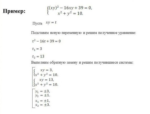
The example shows that by introducing a new variable t, it was possible to reduce the 1st equation of the system to a standard quadratic trinomial. You can solve a polynomial by finding the discriminant.

It is necessary to find the value of the discriminant using the well-known formula: D = b2 - 4*a*c, where D is the desired discriminant, b, a, c are the factors of the polynomial. In the given example, a=1, b=16, c=39, therefore D=100. If the discriminant is greater than zero, then there are two solutions: t = -b±√D / 2*a, if the discriminant is less than zero, then there is one solution: x = -b / 2*a.

The solution for the resulting systems is found by the addition method.

Visual method for solving systems

Suitable for 3 equation systems. The method consists in constructing graphs of each equation included in the system on the coordinate axis. The coordinates of the intersection points of the curves will be the general solution of the system.

The graphical method has a number of nuances. Let's look at several examples of solving systems of linear equations in a visual way.

As can be seen from the example, for each line two points were constructed, the values ​​of the variable x were chosen arbitrarily: 0 and 3. Based on the values ​​of x, the values ​​for y were found: 3 and 0. Points with coordinates (0, 3) and (3, 0) were marked on the graph and connected by a line.

The steps must be repeated for the second equation. The point of intersection of the lines is the solution of the system.

The following example requires finding a graphical solution to a system of linear equations: 0.5x-y+2=0 and 0.5x-y-1=0.

As can be seen from the example, the system has no solution, because the graphs are parallel and do not intersect along their entire length.

The systems from examples 2 and 3 are similar, but when constructed it becomes obvious that their solutions are different. It should be remembered that it is not always possible to say whether a system has a solution or not; it is always necessary to construct a graph.

The matrix and its varieties

Matrices are used to concisely write a system of linear equations. A matrix is ​​a special type of table filled with numbers. n*m has n - rows and m - columns.

A matrix is ​​square when the number of columns and rows are equal. A matrix-vector is a matrix of one column with an infinitely possible number of rows. A matrix with ones along one of the diagonals and other zero elements is called identity.

An inverse matrix is ​​a matrix when multiplied by which the original one turns into a unit matrix; such a matrix exists only for the original square one.

Rules for converting a system of equations into a matrix

In relation to systems of equations, the coefficients and free terms of the equations are written as matrix numbers; one equation is one row of the matrix.

A matrix row is said to be nonzero if at least one element of the row is not zero. Therefore, if in any of the equations the number of variables differs, then it is necessary to enter zero in place of the missing unknown.

The matrix columns must strictly correspond to the variables. This means that the coefficients of the variable x can be written only in one column, for example the first, the coefficient of the unknown y - only in the second.

When multiplying a matrix, all elements of the matrix are sequentially multiplied by a number.

Options for finding the inverse matrix

The formula for finding the inverse matrix is ​​quite simple: K -1 = 1 / |K|, where K -1 is the inverse matrix, and |K| is the determinant of the matrix. |K| must not be equal to zero, then the system has a solution.

The determinant is easily calculated for a two-by-two matrix; you just need to multiply the diagonal elements by each other. For the “three by three” option, there is a formula |K|=a 1 b 2 c 3 + a 1 b 3 c 2 + a 3 b 1 c 2 + a 2 b 3 c 1 + a 2 b 1 c 3 + a 3 b 2 c 1 . You can use the formula, or you can remember that you need to take one element from each row and each column so that the numbers of columns and rows of elements are not repeated in the work.

Solving examples of systems of linear equations using the matrix method

The matrix method of finding a solution allows you to reduce cumbersome entries when solving systems with a large number of variables and equations.

In the example, a nm are the coefficients of the equations, the matrix is ​​a vector x n are variables, and b n are free terms.

Solving systems using the Gaussian method

In higher mathematics, the Gaussian method is studied together with the Cramer method, and the process of finding solutions to systems is called the Gauss-Cramer solution method. These methods are used to find variables of systems with a large number of linear equations.

The Gauss method is very similar to solutions by substitution and algebraic addition, but is more systematic. In the school course, the solution by the Gaussian method is used for systems of 3 and 4 equations. The purpose of the method is to reduce the system to the form of an inverted trapezoid. By means of algebraic transformations and substitutions, the value of one variable is found in one of the equations of the system. The second equation is an expression with 2 unknowns, while 3 and 4 are, respectively, with 3 and 4 variables.

After bringing the system to the described form, the further solution is reduced to the sequential substitution of known variables into the equations of the system.

In school textbooks for grade 7, an example of a solution by the Gauss method is described as follows:

As can be seen from the example, at step (3) two equations were obtained: 3x 3 -2x 4 =11 and 3x 3 +2x 4 =7. Solving any of the equations will allow you to find out one of the variables x n.

Theorem 5, which is mentioned in the text, states that if one of the equations of the system is replaced by an equivalent one, then the resulting system will also be equivalent to the original one.

The Gaussian method is difficult for middle school students to understand, but it is one of the most interesting ways to develop the ingenuity of children enrolled in advanced learning programs in math and physics classes.

For ease of recording, calculations are usually done as follows:

The coefficients of the equations and free terms are written in the form of a matrix, where each row of the matrix corresponds to one of the equations of the system. separates the left side of the equation from the right. Roman numerals indicate the numbers of equations in the system.

First, write down the matrix to be worked with, then all the actions carried out with one of the rows. The resulting matrix is ​​written after the "arrow" sign and the necessary algebraic operations are continued until the result is achieved.

The result should be a matrix in which one of the diagonals is equal to 1, and all other coefficients are equal to zero, that is, the matrix is ​​reduced to a unit form. We must not forget to perform calculations with numbers on both sides of the equation.

This recording method is less cumbersome and allows you not to be distracted by listing numerous unknowns.

The free use of any solution method will require care and some experience. Not all methods are of an applied nature. Some methods of finding solutions are more preferable in a particular area of ​​human activity, while others exist for educational purposes.

Learning to solve equations is one of the main tasks that algebra poses for students. Starting with the simplest, when it consists of one unknown, and moving on to more and more complex ones. If you have not mastered the actions that need to be performed with equations from the first group, it will be difficult to understand the others.

To continue the conversation, you need to agree on notation.

General form of a linear equation with one unknown and the principle of its solution

Any equation that can be written like this:

a * x = b,

called linear. This is the general formula. But often in assignments linear equations are written in implicit form. Then it is necessary to perform identical transformations to obtain a generally accepted notation. These actions include:

• opening parentheses;
• moving all terms with a variable value to the left side of the equality, and the rest to the right;
• reduction of similar terms.

In the case where an unknown quantity is in the denominator of a fraction, it is necessary to determine its values ​​at which the expression will not make sense. In other words, you need to know the domain of definition of the equation.

The principle by which all linear equations are solved comes down to dividing the value on the right side of the equation by the coefficient in front of the variable. That is, “x” will be equal to b/a.

Special cases of linear equations and their solutions

During reasoning, moments may arise when linear equations take on one of the special forms. Each of them has a specific solution.

In the first situation:

a * x = 0, and a ≠ 0.

The solution to such an equation will always be x = 0.

In the second case, “a” takes the value equal to zero:

0 * x = 0.

The answer to such an equation will be any number. That is, it has an infinite number of roots.

The third situation looks like this:

0 * x = in, where in ≠ 0.

This equation doesn't make sense. Because there are no roots that satisfy it.

General view of a linear equation with two variables

From its name it becomes clear that there are already two unknown quantities in it. Linear equations in two variables look like this:

a * x + b * y = c.

Since there are two unknowns in the record, the answer will look like a pair of numbers. That is, it is not enough to specify only one value. This will be an incomplete answer. A pair of quantities for which the equation becomes an identity is a solution to the equation. Moreover, in the answer, the variable that comes first in the alphabet is always written down first. Sometimes they say that these numbers satisfy him. Moreover, there can be an infinite number of such pairs.

How to solve a linear equation with two unknowns?

To do this, you just need to select any pair of numbers that turns out to be correct. For simplicity, you can take one of the unknowns equal to some prime number, and then find the second.

When solving, you often have to perform steps to simplify the equation. They are called identity transformations. Moreover, the following properties are always true for equations:

• each term can be moved to the opposite part of the equality by replacing its sign with the opposite one;
• The left and right sides of any equation are allowed to be divided by the same number, as long as it is not equal to zero.

Examples of tasks with linear equations

First task. Solve linear equations: 4x = 20, 8(x - 1) + 2x = 2(4 - 2x); (5x + 15) / (x + 4) = 4; (5x + 15) / (x + 3) = 4.

In the equation that comes first on this list, simply divide 20 by 4. The result will be 5. This is the answer: x = 5.

The third equation requires that an identity transformation be performed. It will consist of opening the brackets and bringing similar terms. After the first step, the equation will take the form: 8x - 8 + 2x = 8 - 4x. Then you need to move all the unknowns to the left side of the equation, and the rest to the right. The equation will look like this: 8x + 2x + 4x = 8 + 8. After adding similar terms: 14x = 16. Now it looks the same as the first one, and its solution is easy to find. The answer will be x=8/7. But in mathematics you are supposed to isolate the whole part from an improper fraction. Then the result will be transformed, and “x” will be equal to one whole and one seventh.

In the remaining examples, the variables are in the denominator. This means that you first need to find out at what values ​​the equations are defined. To do this, you need to exclude numbers at which the denominators go to zero. In the first example it is “-4”, in the second it is “-3”. That is, these values ​​​​need to be excluded from the answer. After this, you need to multiply both sides of the equality by the expressions in the denominator.

Opening the brackets and bringing similar terms, in the first of these equations we get: 5x + 15 = 4x + 16, and in the second 5x + 15 = 4x + 12. After transformations, the solution to the first equation will be x = -1. The second turns out to be equal to “-3”, which means that the latter has no solutions.

Second task. Solve the equation: -7x + 2y = 5.

Suppose that the first unknown x = 1, then the equation will take the form -7 * 1 + 2y = 5. Moving the factor “-7” to the right side of the equality and changing its sign to plus, it turns out that 2y = 12. This means y =6. Answer: one of the solutions to the equation x = 1, y = 6.

General form of inequality with one variable

All possible situations for inequalities are presented here:

• a * x > b;
• a * x< в;
• a * x ≥b;
• a * x ≤в.

In general, it looks like a simple linear equation, only the equal sign is replaced by an inequality.

Rules for identity transformations of inequality

Just like linear equations, inequalities can be modified according to certain laws. They boil down to the following:

1. any alphabetic or numerical expression can be added to the left and right sides of the inequality, and the sign of the inequality remains the same;
2. you can also multiply or divide by the same positive number, this again does not change the sign;
3. When multiplying or dividing by the same negative number, the equality will remain true provided that the inequality sign is reversed.

General view of double inequalities

The following inequalities can be presented in problems:

• V< а * х < с;
• c ≤ a * x< с;
• V< а * х ≤ с;
• c ≤ a * x ≤ c.

It is called double because it is limited by inequality signs on both sides. It is solved using the same rules as ordinary inequalities. And finding the answer comes down to a series of identical transformations. Until the simplest is obtained.

Features of solving double inequalities

The first of them is its image on the coordinate axis. There is no need to use this method for simple inequalities. But in difficult cases it may simply be necessary.

To depict an inequality, you need to mark on the axis all the points that were obtained during the reasoning. These are invalid values, which are indicated by punctured dots, and values ​​from inequalities obtained after transformations. Here, too, it is important to draw the dots correctly. If the inequality is strict, that is< или >, then these values ​​are punched out. In non-strict inequalities, the points must be shaded.

Then it is necessary to indicate the meaning of the inequalities. This can be done using shading or arcs. Their intersection will indicate the answer.

The second feature is related to its recording. There are two options offered here. The first is ultimate inequality. The second is in the form of intervals. It happens with him that difficulties arise. The answer in spaces always looks like a variable with a membership sign and parentheses with numbers. Sometimes there are several spaces, then between the brackets you need to write the symbol “and”. These signs look like this: ∈ and ∩. Spacing brackets also play a role. The round one is placed when the point is excluded from the answer, and the rectangular one includes this value. The infinity sign is always in parentheses.

Examples of solving inequalities

1. Solve the inequality 7 - 5x ≥ 37.

After simple transformations, we get: -5x ≥ 30. Dividing by “-5” we can get the following expression: x ≤ -6. This is already the answer, but it can be written in another way: x ∈ (-∞; -6].

2. Solve double inequality -4< 2x + 6 ≤ 8.

First you need to subtract 6 everywhere. You get: -10< 2x ≤ 2. Теперь нужно разделить на 2. Неравенство примет вид: -5 < x ≤ 1. Изобразив ответ на числовой оси, сразу можно понять, что результатом будет промежуток от -5 до 1. Причем первая точка исключена, а вторая включена. То есть ответ у неравенства такой: х ∈ (-5; 1].