Systems of equations are widely used in the economic sector for mathematical modeling of various processes. For example, when solving problems of production management and planning, logistics routes (transport problem) or equipment placement.
Systems of equations are used not only in mathematics, but also in physics, chemistry and biology, when solving problems of finding population size.
A system of linear equations is two or more equations with several variables for which it is necessary to find a common solution. Such a sequence of numbers for which all equations become true equalities or prove that the sequence does not exist.
Linear equation
Equations of the form ax+by=c are called linear. The designations x, y are the unknowns whose value must be found, b, a are the coefficients of the variables, c is the free term of the equation.
Solving an equation by plotting it will look like a straight line, all points of which are solutions to the polynomial.
Types of systems of linear equations
The simplest examples are considered to be systems of linear equations with two variables X and Y.
F1(x, y) = 0 and F2(x, y) = 0, where F1,2 are functions and (x, y) are function variables.
Solve system of equations - this means finding values (x, y) at which the system turns into a true equality or establishing that suitable values of x and y do not exist.
A pair of values (x, y), written as the coordinates of a point, is called a solution to a system of linear equations.
If systems have one common solution or no solution exists, they are called equivalent.
Homogeneous systems of linear equations are systems whose right-hand side is equal to zero. If the right part after the equal sign has a value or is expressed by a function, such a system is heterogeneous.
The number of variables can be much more than two, then we should talk about an example of a system of linear equations with three or more variables.
When faced with systems, schoolchildren assume that the number of equations must necessarily coincide with the number of unknowns, but this is not the case. The number of equations in the system does not depend on the variables; there can be as many of them as desired.
Simple and complex methods for solving systems of equations
There is no general analytical method for solving such systems; all methods are based on numerical solutions. The school mathematics course describes in detail such methods as permutation, algebraic addition, substitution, as well as graphical and matrix methods, solution by the Gaussian method.
The main task when teaching solution methods is to teach how to correctly analyze the system and find the optimal solution algorithm for each example. The main thing is not to memorize a system of rules and actions for each method, but to understand the principles of using a particular method
Solving examples of systems of linear equations in the 7th grade general education curriculum is quite simple and explained in great detail. In any mathematics textbook, this section is given enough attention. Solving examples of systems of linear equations using the Gauss and Cramer method is studied in more detail in the first years of higher education.
Solving systems using the substitution method
The actions of the substitution method are aimed at expressing the value of one variable in terms of the second. The expression is substituted into the remaining equation, then it is reduced to a form with one variable. The action is repeated depending on the number of unknowns in the system
Let us give a solution to an example of a system of linear equations of class 7 using the substitution method:

As can be seen from the example, the variable x was expressed through F(X) = 7 + Y. The resulting expression, substituted into the 2nd equation of the system in place of X, helped to obtain one variable Y in the 2nd equation. Solving this example is easy and allows you to get the Y value. The last step is to check the obtained values.
It is not always possible to solve an example of a system of linear equations by substitution. The equations can be complex and expressing the variable in terms of the second unknown will be too cumbersome for further calculations. When there are more than 3 unknowns in the system, solving by substitution is also inappropriate.
Solution of an example of a system of linear inhomogeneous equations:

Solution using algebraic addition
When searching for solutions to systems using the addition method, equations are added term by term and multiplied by various numbers. The ultimate goal of mathematical operations is an equation in one variable.

Application of this method requires practice and observation. Solving a system of linear equations using the addition method when there are 3 or more variables is not easy. Algebraic addition is convenient to use when equations contain fractions and decimals.
Solution algorithm:
- Multiply both sides of the equation by a certain number. As a result of the arithmetic operation, one of the coefficients of the variable should become equal to 1.
- Add the resulting expression term by term and find one of the unknowns.
- Substitute the resulting value into the 2nd equation of the system to find the remaining variable.
Method of solution by introducing a new variable
A new variable can be introduced if the system requires finding a solution for no more than two equations; the number of unknowns should also be no more than two.
The method is used to simplify one of the equations by introducing a new variable. The new equation is solved for the introduced unknown, and the resulting value is used to determine the original variable.
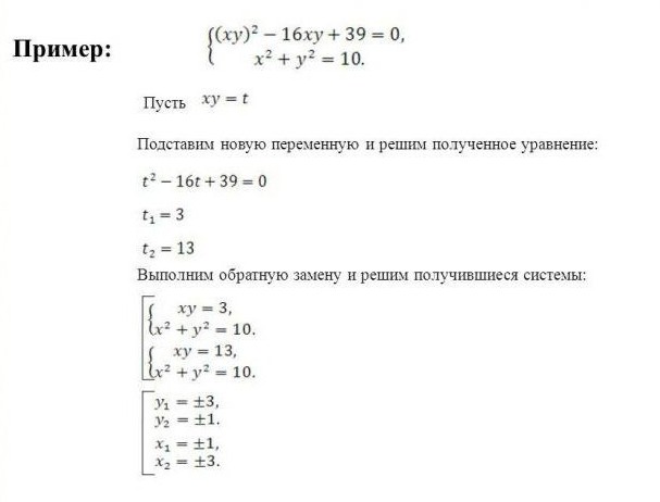
The example shows that by introducing a new variable t, it was possible to reduce the 1st equation of the system to a standard quadratic trinomial. You can solve a polynomial by finding the discriminant.
It is necessary to find the value of the discriminant using the well-known formula: D = b2 - 4*a*c, where D is the desired discriminant, b, a, c are the factors of the polynomial. In the given example, a=1, b=16, c=39, therefore D=100. If the discriminant is greater than zero, then there are two solutions: t = -b±√D / 2*a, if the discriminant is less than zero, then there is one solution: x = -b / 2*a.
The solution for the resulting systems is found by the addition method.
Visual method for solving systems
Suitable for 3 equation systems. The method consists in constructing graphs of each equation included in the system on the coordinate axis. The coordinates of the intersection points of the curves will be the general solution of the system.
The graphical method has a number of nuances. Let's look at several examples of solving systems of linear equations in a visual way.

As can be seen from the example, for each line two points were constructed, the values of the variable x were chosen arbitrarily: 0 and 3. Based on the values of x, the values for y were found: 3 and 0. Points with coordinates (0, 3) and (3, 0) were marked on the graph and connected by a line.
The steps must be repeated for the second equation. The point of intersection of the lines is the solution of the system.
The following example requires finding a graphical solution to a system of linear equations: 0.5x-y+2=0 and 0.5x-y-1=0.

As can be seen from the example, the system has no solution, because the graphs are parallel and do not intersect along their entire length.

The systems from examples 2 and 3 are similar, but when constructed it becomes obvious that their solutions are different. It should be remembered that it is not always possible to say whether a system has a solution or not; it is always necessary to construct a graph.
The matrix and its varieties
Matrices are used to concisely write a system of linear equations. A matrix is a special type of table filled with numbers. n*m has n - rows and m - columns.
A matrix is square when the number of columns and rows are equal. A matrix-vector is a matrix of one column with an infinitely possible number of rows. A matrix with ones along one of the diagonals and other zero elements is called identity.
An inverse matrix is a matrix when multiplied by which the original one turns into a unit matrix; such a matrix exists only for the original square one.
Rules for converting a system of equations into a matrix
In relation to systems of equations, the coefficients and free terms of the equations are written as matrix numbers; one equation is one row of the matrix.
A matrix row is said to be nonzero if at least one element of the row is not zero. Therefore, if in any of the equations the number of variables differs, then it is necessary to enter zero in place of the missing unknown.
The matrix columns must strictly correspond to the variables. This means that the coefficients of the variable x can be written only in one column, for example the first, the coefficient of the unknown y - only in the second.
When multiplying a matrix, all elements of the matrix are sequentially multiplied by a number.
Options for finding the inverse matrix
The formula for finding the inverse matrix is quite simple: K -1 = 1 / |K|, where K -1 is the inverse matrix, and |K| is the determinant of the matrix. |K| must not be equal to zero, then the system has a solution.
The determinant is easily calculated for a two-by-two matrix; you just need to multiply the diagonal elements by each other. For the “three by three” option, there is a formula |K|=a 1 b 2 c 3 + a 1 b 3 c 2 + a 3 b 1 c 2 + a 2 b 3 c 1 + a 2 b 1 c 3 + a 3 b 2 c 1 . You can use the formula, or you can remember that you need to take one element from each row and each column so that the numbers of columns and rows of elements are not repeated in the work.
Solving examples of systems of linear equations using the matrix method
The matrix method of finding a solution allows you to reduce cumbersome entries when solving systems with a large number of variables and equations.

In the example, a nm are the coefficients of the equations, the matrix is a vector x n are variables, and b n are free terms.


Solving systems using the Gaussian method
In higher mathematics, the Gaussian method is studied together with the Cramer method, and the process of finding solutions to systems is called the Gauss-Cramer solution method. These methods are used to find variables of systems with a large number of linear equations.
The Gauss method is very similar to solutions by substitution and algebraic addition, but is more systematic. In the school course, the solution by the Gaussian method is used for systems of 3 and 4 equations. The purpose of the method is to reduce the system to the form of an inverted trapezoid. By means of algebraic transformations and substitutions, the value of one variable is found in one of the equations of the system. The second equation is an expression with 2 unknowns, while 3 and 4 are, respectively, with 3 and 4 variables.
After bringing the system to the described form, the further solution is reduced to the sequential substitution of known variables into the equations of the system.
In school textbooks for grade 7, an example of a solution by the Gauss method is described as follows:

As can be seen from the example, at step (3) two equations were obtained: 3x 3 -2x 4 =11 and 3x 3 +2x 4 =7. Solving any of the equations will allow you to find out one of the variables x n.

Theorem 5, which is mentioned in the text, states that if one of the equations of the system is replaced by an equivalent one, then the resulting system will also be equivalent to the original one.
The Gaussian method is difficult for middle school students to understand, but it is one of the most interesting ways to develop the ingenuity of children enrolled in advanced math and physics classes.
For ease of recording, calculations are usually done as follows:

The coefficients of the equations and free terms are written in the form of a matrix, where each row of the matrix corresponds to one of the equations of the system. separates the left side of the equation from the right. Roman numerals indicate the numbers of equations in the system.
First, write down the matrix to be worked with, then all the actions carried out with one of the rows. The resulting matrix is written after the "arrow" sign and the necessary algebraic operations are continued until the result is achieved.
The result should be a matrix in which one of the diagonals is equal to 1, and all other coefficients are equal to zero, that is, the matrix is reduced to a unit form. We must not forget to perform calculations with numbers on both sides of the equation.
This recording method is less cumbersome and allows you not to be distracted by listing numerous unknowns.
The free use of any solution method will require care and some experience. Not all methods are of an applied nature. Some methods of finding solutions are more preferable in a particular area of human activity, while others exist for educational purposes.
In this article we will consider the principle of solving such equations as linear equations. Let's write down the definition of these equations and set the general form. We will analyze all the conditions for finding solutions to linear equations, using, among other things, practical examples.
Please note that the material below contains information on linear equations with one variable. Linear equations in two variables are discussed in a separate article.
Yandex.RTB R-A-339285-1
What is a linear equation
Definition 1Linear equation is an equation written as follows:
a x = b, Where x– variable, a And b- some numbers.
This formulation was used in the algebra textbook (7th grade) by Yu.N. Makarychev.
Example 1
Examples of linear equations would be:
3 x = 11(equation with one variable x at a = 5 And b = 10);
− 3 , 1 y = 0 ( linear equation with variable y, Where a = - 3, 1 And b = 0);
x = − 4 And − x = 5.37(linear equations, where the number a written explicitly and equal to 1 and - 1, respectively. For the first equation b = - 4 ; for the second - b = 5.37) and so on.
Different educational materials may have different definitions. For example, Vilenkin N.Ya. Linear equations also include those equations that can be transformed into the form a x = b by transferring terms from one part to another with a change of sign and bringing similar terms. If we follow this interpretation, the equation 5 x = 2 x + 6 – also linear.
But the algebra textbook (7th grade) by Mordkovich A.G. gives the following description:
Definition 2
A linear equation in one variable x is an equation of the form a x + b = 0, Where a And b– some numbers called coefficients of a linear equation.
Example 2
An example of linear equations of this type could be:
3 x − 7 = 0 (a = 3 , b = − 7) ;
1, 8 y + 7, 9 = 0 (a = 1, 8, b = 7, 9).
But there are also examples of linear equations that we have already used above: of the form a x = b, For example, 6 x = 35.
We will immediately agree that in this article, by a linear equation with one variable we will understand the equation written a x + b = 0, Where x– variable; a, b – coefficients. We see this form of a linear equation as the most justified, since linear equations are algebraic equations of the first degree. And the other equations indicated above, and the equations given by equivalent transformations in the form a x + b = 0, we define as equations that reduce to linear equations.
With this approach, the equation 5 x + 8 = 0 is linear, and 5 x = − 8- an equation that reduces to a linear one.
Principle of solving linear equations
Let's look at how to determine whether a given linear equation will have roots and, if so, how many and how to determine them.
Definition 3
The fact of the presence of roots of a linear equation is determined by the values of the coefficients a And b. Let's write down these conditions:
- at a ≠ 0 linear equation has a single root x = - b a ;
- at a = 0 And b ≠ 0 a linear equation has no roots;
- at a = 0 And b = 0 a linear equation has infinitely many roots. Essentially, in this case, any number can become the root of a linear equation.
Let's give an explanation. We know that in the process of solving an equation it is possible to transform a given equation into one that is equivalent to it, which means that it has the same roots as the original equation, or also has no roots. We can make the following equivalent transformations:
- transfer a term from one part to another, changing the sign to the opposite;
- multiply or divide both sides of an equation by the same number that is not zero.
Thus, we transform the linear equation a x + b = 0, moving the term b from the left side to the right side with a change of sign. We get: a · x = − b .
So, we divide both sides of the equation by a non-zero number A, resulting in an equality of the form x = - b a . That is, when a ≠ 0, original equation a x + b = 0 is equivalent to the equality x = - b a, in which the root - b a is obvious.
By contradiction it is possible to demonstrate that the root found is the only one. Let us designate the found root - b a as x 1 . Let us assume that there is another root of the linear equation with the designation x 2 . And of course: x 2 ≠ x 1, and this, in turn, based on the definition of equal numbers through the difference, is equivalent to the condition x 1 − x 2 ≠ 0 . Taking into account the above, we can create the following equalities by substituting the roots:
a x 1 + b = 0 and a x 2 + b = 0.
The property of numerical equalities makes it possible to perform term-by-term subtraction of parts of equalities:
a x 1 + b − (a x 2 + b) = 0 − 0, from here: a · (x 1 − x 2) + (b − b) = 0 and onwards a · (x 1 − x 2) = 0 . Equality a · (x 1 − x 2) = 0 is incorrect because it was previously specified that a ≠ 0 And x 1 − x 2 ≠ 0 . The resulting contradiction serves as proof that when a ≠ 0 linear equation a x + b = 0 has only one root.
Let us justify two more clauses of the conditions containing a = 0 .
When a = 0 linear equation a x + b = 0 will be written as 0 x + b = 0. The property of multiplying a number by zero gives us the right to assert that whatever number is taken as x, substituting it into equality 0 x + b = 0, we get b = 0 . The equality is valid for b = 0; in other cases, when b ≠ 0, equality becomes false.
So when a = 0 and b = 0 , any number can become the root of a linear equation a x + b = 0, since when these conditions are met, substituting instead x any number, we get the correct numerical equality 0 = 0 . When a = 0 And b ≠ 0 linear equation a x + b = 0 will not have roots at all, since when the specified conditions are met, substituting instead x any number, we get an incorrect numerical equality b = 0.
All the above considerations give us the opportunity to write down an algorithm that makes it possible to find a solution to any linear equation:
- by the type of record we determine the values of the coefficients a And b and analyze them;
- at a = 0 And b = 0 the equation will have infinitely many roots, i.e. any number will become the root of the given equation;
- at a = 0 And b ≠ 0
- at a, different from zero, we begin searching for the only root of the original linear equation:
- let's move the coefficient b to the right side with a change of sign to the opposite, bringing the linear equation to the form a · x = − b ;
- divide both sides of the resulting equality by the number a, which will give us the desired root of the given equation: x = - b a.
Actually, the described sequence of actions is the answer to the question of how to find a solution to a linear equation.
Finally, let us clarify that equations of the form a x = b are solved using a similar algorithm with the only difference that the number b in such a notation has already been transferred to the required part of the equation, and with a ≠ 0 you can immediately divide the parts of an equation by a number a.
Thus, to find a solution to the equation a x = b, we use the following algorithm:
- at a = 0 And b = 0 the equation will have infinitely many roots, i.e. any number can become its root;
- at a = 0 And b ≠ 0 the given equation will have no roots;
- at a, not equal to zero, both sides of the equation are divided by the number a, which makes it possible to find the only root that is equal to b a.
Examples of solving linear equations
Example 3Linear equation needs to be solved 0 x − 0 = 0.
Solution
By writing the given equation we see that a = 0 And b = − 0(or b = 0, which is the same). Thus, a given equation can have an infinite number of roots or any number.
Answer: x– any number.
Example 4
It is necessary to determine whether the equation has roots 0 x + 2, 7 = 0.
Solution
From the record we determine that a = 0, b = 2, 7. Thus, the given equation will have no roots.
Answer: the original linear equation has no roots.
Example 5
Given a linear equation 0.3 x − 0.027 = 0. It needs to be resolved.
Solution
By writing the equation we determine that a = 0, 3; b = - 0.027, which allows us to assert that the given equation has a single root.
Following the algorithm, we move b to the right side of the equation, changing the sign, we get: 0.3 x = 0.027. Next, we divide both sides of the resulting equality by a = 0, 3, then: x = 0, 027 0, 3.
Let's divide decimal fractions:
0.027 0.3 = 27 300 = 3 9 3 100 = 9 100 = 0.09
The result obtained is the root of the given equation.
Let us briefly write the solution as follows:
0.3 x - 0.027 = 0.0.3 x = 0.027, x = 0.027 0.3, x = 0.09.
Answer: x = 0.09.
For clarity, we present the solution to the writing equation a x = b.
Example N
The given equations are: 1) 0 x = 0 ; 2) 0 x = − 9 ; 3) - 3 8 x = - 3 3 4 . They need to be resolved.
Solution
All given equations correspond to the entry a x = b. Let's look at it one by one.
In the equation 0 x = 0, a = 0 and b = 0, which means: any number can be the root of this equation.
In the second equation 0 x = − 9: a = 0 and b = − 9, thus, this equation will have no roots.
Based on the form of the last equation - 3 8 · x = - 3 3 4, we write the coefficients: a = - 3 8, b = - 3 3 4, i.e. the equation has a single root. Let's find him. Let's divide both sides of the equation by a, resulting in: x = - 3 3 4 - 3 8. Let's simplify the fraction by applying the rule for dividing negative numbers, followed by converting the mixed number into an ordinary fraction and dividing ordinary fractions:
3 3 4 - 3 8 = 3 3 4 3 8 = 15 4 3 8 = 15 4 8 3 = 15 8 4 3 = 10
Let us briefly write the solution as follows:
3 8 · x = - 3 3 4 , x = - 3 3 4 - 3 8 , x = 10 .
Answer: 1) x– any number, 2) the equation has no roots, 3) x = 10.
If you notice an error in the text, please highlight it and press Ctrl+Enter
- An equality with a variable is called an equation.
- Solving an equation means finding its many roots. An equation may have one, two, several, many roots, or none at all.
- Each value of a variable at which a given equation turns into a true equality is called a root of the equation.
- Equations that have the same roots are called equivalent equations.
- Any term of the equation can be transferred from one part of the equality to another, while changing the sign of the term to the opposite.
- If both sides of an equation are multiplied or divided by the same non-zero number, you get an equation equivalent to the given equation.
Examples. Solve the equation.
1. 1.5x+4 = 0.3x-2.
1.5x-0.3x = -2-4. We collected the terms containing the variable on the left side of the equality, and the free terms on the right side of the equality. In this case, the following property was used:
1.2x = -6. Similar terms were given according to the rule:
x = -6 : 1.2. Both sides of the equality were divided by the coefficient of the variable, since
x = -5. Divide according to the rule for dividing a decimal fraction by a decimal fraction:
To divide a number by a decimal fraction, you need to move the commas in the dividend and divisor as many digits to the right as there are after the decimal point in the divisor, and then divide by a natural number:
6 : 1,2 = 60 : 12 = 5.
Answer: 5.
2. 3∙ (2x-9) = 4 ∙ (x-4).
6x-27 = 4x-16. We opened the brackets using the distributive law of multiplication relative to subtraction: (a-b) ∙ c = a ∙ c-b ∙ c.
6x-4x = -16+27. We collected the terms containing the variable on the left side of the equality, and the free terms on the right side of the equality. In this case, the following property was used: any term of the equation can be transferred from one part of the equality to another, thereby changing the sign of the term to the opposite.
2x = 11. Similar terms were given according to the rule: to bring similar terms, you need to add their coefficients and multiply the resulting result by their common letter part (i.e., add their common letter part to the result obtained).
x = 11 : 2. Both sides of the equality were divided by the coefficient of the variable, since If both sides of the equation are multiplied or divided by the same non-zero number, you get an equation equivalent to the given equation.
Answer: 5,5.
3. 7x- (3+2x)=x-9.
7x-3-2x = x-9. We opened the brackets according to the rule for opening brackets preceded by a “-” sign: if there is a “-” sign in front of the brackets, then remove the brackets, the “-” sign and write the terms in the brackets with opposite signs.
7x-2x-x = -9+3. We collected the terms containing the variable on the left side of the equality, and the free terms on the right side of the equality. In this case, the following property was used: any term of the equation can be transferred from one part of the equality to another, thereby changing the sign of the term to the opposite.
4x = -6. Similar terms were given according to the rule: to bring similar terms, you need to add their coefficients and multiply the resulting result by their common letter part (i.e., add their common letter part to the result obtained).
x = -6 : 4. Both sides of the equality were divided by the coefficient of the variable, since If both sides of the equation are multiplied or divided by the same non-zero number, you get an equation equivalent to the given equation.
Answer: -1,5.
3 ∙ (x-5) = 7 ∙ 12 — 4 ∙ (2x-11). We multiplied both sides of the equation by 12 - the lowest common denominator for the denominators of these fractions.
3x-15 = 84-8x+44. We opened the brackets using the distributive law of multiplication relative to subtraction: In order to multiply the difference of two numbers by a third number, you can separately multiply the minuend and separately subtract by the third number, and then subtract the second result from the first result, i.e.(a-b) ∙ c = a ∙ c-b ∙ c.
3x+8x = 84+44+15. We collected the terms containing the variable on the left side of the equality, and the free terms on the right side of the equality. In this case, the following property was used: any term of the equation can be transferred from one part of the equality to another, thereby changing the sign of the term to the opposite.
Linear equations. Solution, examples.
Attention!
There are additional
materials in Special Section 555.
For those who are very "not very..."
And for those who “very much…”)
Linear equations.
Linear equations are not the most difficult topic in school mathematics. But there are some tricks there that can puzzle even a trained student. Let's figure it out?)
Typically a linear equation is defined as an equation of the form:
ax + b = 0 Where a and b– any numbers.
2x + 7 = 0. Here a=2, b=7
0.1x - 2.3 = 0 Here a=0.1, b=-2.3
12x + 1/2 = 0 Here a=12, b=1/2
Nothing complicated, right? Especially if you don't notice the words: "where a and b are any numbers"... And if you notice and carelessly think about it?) After all, if a=0, b=0(any numbers are possible?), then we get a funny expression:
But that's not all! If, say, a=0, A b=5, This turns out to be something completely absurd:
Which is annoying and undermines confidence in mathematics, yes...) Especially during exams. But out of these strange expressions you also need to find X! Which doesn't exist at all. And, surprisingly, this X is very easy to find. We will learn to do this. In this lesson.
How to recognize a linear equation by its appearance? It depends on the appearance.) The trick is that linear equations are not only equations of the form ax + b = 0 , but also any equations that can be reduced to this form by transformations and simplifications. And who knows whether it comes down or not?)
A linear equation can be clearly recognized in some cases. Let's say, if we have an equation in which there are only unknowns to the first degree and numbers. And in the equation there is no fractions divided by unknown , it is important! And division by number, or a numerical fraction - that's welcome! For example:
This is a linear equation. There are fractions here, but there are no x's in the square, cube, etc., and no x's in the denominators, i.e. No division by x. And here is the equation

cannot be called linear. Here the X's are all in the first degree, but there are division by expression with x. After simplifications and transformations, you can get a linear equation, a quadratic equation, or anything you want.
It turns out that it is impossible to recognize the linear equation in some complicated example until you almost solve it. This is upsetting. But in assignments, as a rule, they don’t ask about the form of the equation, right? The assignments ask for equations decide. This makes me happy.)
Solving linear equations. Examples.
The entire solution of linear equations consists of identical transformations of the equations. By the way, these transformations (two of them!) are the basis of the solutions all equations of mathematics. In other words, the solution any the equation begins with these very transformations. In the case of linear equations, it (the solution) is based on these transformations and ends with a full answer. It makes sense to follow the link, right?) Moreover, there are also examples of solving linear equations there.
First, let's look at the simplest example. Without any pitfalls. Suppose we need to solve this equation.
x - 3 = 2 - 4x
This is a linear equation. The X's are all in the first power, there is no division by X's. But, in fact, it doesn’t matter to us what kind of equation it is. We need to solve it. The scheme here is simple. Collect everything with X's on the left side of the equation, everything without X's (numbers) on the right.
To do this you need to transfer - 4x to the left side, with a change of sign, of course, and - 3 - to the right. By the way, this is the first identical transformation of equations. Surprised? This means that you didn’t follow the link, but in vain...) We get:
x + 4x = 2 + 3
Here are similar ones, we consider:
What do we need for complete happiness? Yes, so that there is a pure X on the left! Five is in the way. Getting rid of the five with the help the second identical transformation of equations. Namely, we divide both sides of the equation by 5. We get a ready answer:
An elementary example, of course. This is for warming up.) It’s not very clear why I remembered identical transformations here? OK. Let's take the bull by the horns.) Let's decide something more solid.
For example, here's the equation:

Where do we start? With X's - to the left, without X's - to the right? Could be so. Small steps along a long road. Or you can do it right away, in a universal and powerful way. If, of course, you have identical transformations of equations in your arsenal.
I ask you a key question: What do you dislike most about this equation?
95 out of 100 people will answer: fractions ! The answer is correct. So let's get rid of them. Therefore, we start immediately with second identity transformation. What do you need to multiply the fraction on the left by so that the denominator is completely reduced? That's right, at 3. And on the right? By 4. But mathematics allows us to multiply both sides by the same number. How can we get out? Let's multiply both sides by 12! Those. to a common denominator. Then both the three and the four will be reduced. Don't forget that you need to multiply each part entirely. Here's what the first step looks like:

Expanding the brackets:

Note! Numerator (x+2) I put it in brackets! This is because when multiplying fractions, the entire numerator is multiplied! Now you can reduce fractions:
Expand the remaining brackets:
Not an example, but sheer pleasure!) Now let’s remember a spell from elementary school: with an X - to the left, without an X - to the right! And apply this transformation:
Here are some similar ones:
And divide both parts by 25, i.e. apply the second transformation again:

That's all. Answer: X=0,16
Please note: to bring the original confusing equation into a nice form, we used two (just two!) identity transformations– translation left-right with a change of sign and multiplication-division of an equation by the same number. This is a universal method! We will work in this way with any equations! Absolutely anyone. That’s why I tediously repeat about these identical transformations all the time.)
As you can see, the principle of solving linear equations is simple. We take the equation and simplify it using identical transformations until we get the answer. The main problems here are in the calculations, not in the principle of the solution.
But... There are such surprises in the process of solving the most elementary linear equations that they can drive you into a strong stupor...) Fortunately, there can only be two such surprises. Let's call them special cases.
Special cases in solving linear equations.
First surprise.
Suppose you come across a very basic equation, something like:
2x+3=5x+5 - 3x - 2
Slightly bored, we move it with an X to the left, without an X - to the right... With a change of sign, everything is perfect... We get:
2x-5x+3x=5-2-3
We count, and... oops!!! We get:
This equality in itself is not objectionable. Zero really is zero. But X is missing! And we must write down in the answer, What is x equal to? Otherwise, the solution doesn't count, right...) Dead end?
Calm! In such doubtful cases, the most general rules can save you. How to solve equations? What does it mean to solve an equation? This means, find all the values of x that, when substituted into the original equation, will give us the correct equality.
But we have true equality already happened! 0=0, how much more accurate?! It remains to figure out at what x's this happens. What values of X can be substituted into original equation if these x's will they still be reduced to zero? Come on?)
Yes!!! X's can be substituted any! Which ones do you want? At least 5, at least 0.05, at least -220. They will still shrink. If you don’t believe me, you can check it.) Substitute any values of X into original equation and calculate. All the time you will get the pure truth: 0=0, 2=2, -7.1=-7.1 and so on.
Here's your answer: x - any number.
The answer can be written in different mathematical symbols, the essence does not change. This is a completely correct and complete answer.
Second surprise.
Let's take the same elementary linear equation and change just one number in it. This is what we will decide:
2x+1=5x+5 - 3x - 2
After the same identical transformations, we get something intriguing:
Like this. We solved a linear equation and got a strange equality. In mathematical terms, we got false equality. But in simple terms, this is not true. Rave. But nevertheless, this nonsense is a very good reason for the correct solution of the equation.)
Again we think based on general rules. What x's, when substituted into the original equation, will give us true equality? Yes, none! There are no such X's. No matter what you put in, everything will be reduced, only nonsense will remain.)
Here's your answer: there are no solutions.
This is also a completely complete answer. In mathematics, such answers are often found.
Like this. Now, I hope, the disappearance of X's in the process of solving any (not just linear) equation will not confuse you at all. This is already a familiar matter.)
Now that we have dealt with all the pitfalls in linear equations, it makes sense to solve them.
If you like this site...
By the way, I have a couple more interesting sites for you.)
You can practice solving examples and find out your level. Testing with instant verification. Let's learn - with interest!)
You can get acquainted with functions and derivatives.
In this video we will analyze a whole set of linear equations that are solved using the same algorithm - that’s why they are called the simplest.
First, let's define: what is a linear equation and which one is called the simplest?
A linear equation is one in which there is only one variable, and only to the first degree.
The simplest equation means the construction:
All other linear equations are reduced to the simplest using the algorithm:
- Expand parentheses, if any;
- Move terms containing a variable to one side of the equal sign, and terms without a variable to the other;
- Give similar terms to the left and right of the equal sign;
- Divide the resulting equation by the coefficient of the variable $x$.
Of course, this algorithm does not always help. The fact is that sometimes after all these machinations the coefficient of the variable $x$ turns out to be equal to zero. In this case, two options are possible:
- The equation has no solutions at all. For example, when something like $0\cdot x=8$ turns out, i.e. on the left is a zero, and on the right is a number other than zero. In the video below we will look at several reasons why this situation is possible.
- The solution is all numbers. The only case when this is possible is when the equation has been reduced to the construction $0\cdot x=0$. It is quite logical that no matter what $x$ we substitute, it will still turn out “zero is equal to zero”, i.e. correct numerical equality.
Now let's see how all this works using real-life examples.
Examples of solving equations
Today we are dealing with linear equations, and only the simplest ones. In general, a linear equation means any equality that contains exactly one variable, and it goes only to the first degree.
Such constructions are solved in approximately the same way:
- First of all, you need to expand the parentheses, if there are any (as in our last example);
- Then bring similar
- Finally, isolate the variable, i.e. move everything connected with the variable—the terms in which it is contained—to one side, and move everything that remains without it to the other side.
Then, as a rule, you need to give similar ones on each side of the resulting equality, and after that all that remains is to divide by the coefficient of “x”, and we will get the final answer.
In theory, this looks nice and simple, but in practice, even experienced high school students can make offensive mistakes in fairly simple linear equations. Typically, errors are made either when opening brackets or when calculating the “pluses” and “minuses”.
In addition, it happens that a linear equation has no solutions at all, or that the solution is the entire number line, i.e. any number. We will look at these subtleties in today's lesson. But we will start, as you already understood, with the simplest tasks.
Scheme for solving simple linear equations
First, let me once again write the entire scheme for solving the simplest linear equations:
- Expand the brackets, if any.
- We isolate the variables, i.e. We move everything that contains “X’s” to one side, and everything without “X’s” to the other.
- We present similar terms.
- We divide everything by the coefficient of “x”.
Of course, this scheme does not always work; there are certain subtleties and tricks in it, and now we will get to know them.
Solving real examples of simple linear equations
Task No. 1
The first step requires us to open the brackets. But they are not in this example, so we skip this step. In the second step we need to isolate the variables. Please note: we are talking only about individual terms. Let's write it down:
We present similar terms on the left and right, but this has already been done here. Therefore, we move on to the fourth step: divide by the coefficient:
\[\frac(6x)(6)=-\frac(72)(6)\]
So we got the answer.
Task No. 2
We can see the parentheses in this problem, so let's expand them:
Both on the left and on the right we see approximately the same design, but let's act according to the algorithm, i.e. separating the variables:
Here are some similar ones:
At what roots does this work? Answer: for any. Therefore, we can write that $x$ is any number.
Task No. 3
The third linear equation is more interesting:
\[\left(6-x \right)+\left(12+x \right)-\left(3-2x \right)=15\]
There are several brackets here, but they are not multiplied by anything, they are simply preceded by different signs. Let's break them down:
We perform the second step already known to us:
\[-x+x+2x=15-6-12+3\]
Let's do the math:
We carry out the last step - divide everything by the coefficient of “x”:
\[\frac(2x)(x)=\frac(0)(2)\]
Things to Remember When Solving Linear Equations
If we ignore too simple tasks, I would like to say the following:
- As I said above, not every linear equation has a solution - sometimes there are simply no roots;
- Even if there are roots, there may be zero among them - there is nothing wrong with that.
Zero is the same number as the others; you shouldn’t discriminate against it in any way or assume that if you get zero, then you did something wrong.
Another feature is related to the opening of brackets. Please note: when there is a “minus” in front of them, we remove it, but in parentheses we change the signs to opposite. And then we can open it using standard algorithms: we will get what we saw in the calculations above.
Understanding this simple fact will help you avoid making stupid and hurtful mistakes in high school, when doing such things is taken for granted.
Solving complex linear equations
Let's move on to more complex equations. Now the constructions will become more complex and when performing various transformations a quadratic function will appear. However, we should not be afraid of this, because if, according to the author’s plan, we are solving a linear equation, then during the transformation process all monomials containing a quadratic function will necessarily cancel.
Example No. 1
Obviously, the first step is to open the brackets. Let's do this very carefully:
Now let's take a look at privacy:
\[-x+6((x)^(2))-6((x)^(2))+x=-12\]
Here are some similar ones:
Obviously, this equation has no solutions, so we’ll write this in the answer:
\[\varnothing\]
or there are no roots.
Example No. 2
We perform the same actions. First step:
Let's move everything with a variable to the left, and without it - to the right:
Here are some similar ones:
Obviously, this linear equation has no solution, so we’ll write it this way:
\[\varnothing\],
or there are no roots.
Nuances of the solution
Both equations are completely solved. Using these two expressions as an example, we were once again convinced that even in the simplest linear equations, everything may not be so simple: there can be either one, or none, or infinitely many roots. In our case, we considered two equations, both simply have no roots.
But I would like to draw your attention to another fact: how to work with parentheses and how to open them if there is a minus sign in front of them. Consider this expression:
Before opening, you need to multiply everything by “X”. Please note: multiplies each individual term. Inside there are two terms - respectively, two terms and multiplied.
And only after these seemingly elementary, but very important and dangerous transformations have been completed, can you open the bracket from the point of view of the fact that there is a minus sign after it. Yes, yes: only now, when the transformations are completed, we remember that there is a minus sign in front of the brackets, which means that everything below simply changes signs. At the same time, the brackets themselves disappear and, most importantly, the front “minus” also disappears.
We do the same with the second equation:
It is not by chance that I pay attention to these small, seemingly insignificant facts. Because solving equations is always a sequence of elementary transformations, where the inability to clearly and competently perform simple actions leads to the fact that high school students come to me and again learn to solve such simple equations.
Of course, the day will come when you will hone these skills to the point of automaticity. You will no longer have to perform so many transformations each time; you will write everything on one line. But while you are just learning, you need to write each action separately.
Solving even more complex linear equations
What we are going to solve now can hardly be called the simplest task, but the meaning remains the same.
Task No. 1
\[\left(7x+1 \right)\left(3x-1 \right)-21((x)^(2))=3\]
Let's multiply all the elements in the first part:
Let's do some privacy:
Here are some similar ones:
Let's complete the last step:
\[\frac(-4x)(4)=\frac(4)(-4)\]
Here is our final answer. And, despite the fact that in the process of solving we had coefficients with a quadratic function, they canceled each other out, which makes the equation linear and not quadratic.
Task No. 2
\[\left(1-4x \right)\left(1-3x \right)=6x\left(2x-1 \right)\]
Let's carefully perform the first step: multiply each element from the first bracket by each element from the second. There should be a total of four new terms after the transformations:
Now let’s carefully perform the multiplication in each term:
Let’s move the terms with “X” to the left, and those without - to the right:
\[-3x-4x+12((x)^(2))-12((x)^(2))+6x=-1\]
Here are similar terms:
Once again we have received the final answer.
Nuances of the solution
The most important note about these two equations is the following: as soon as we begin to multiply brackets that contain more than one term, this is done according to the following rule: we take the first term from the first and multiply with each element from the second; then we take the second element from the first and similarly multiply with each element from the second. As a result, we will have four terms.
About the algebraic sum
With this last example, I would like to remind students what an algebraic sum is. In classical mathematics, by $1-7$ we mean a simple construction: subtract seven from one. In algebra, we mean the following by this: to the number “one” we add another number, namely “minus seven”. This is how an algebraic sum differs from an ordinary arithmetic sum.
As soon as, when performing all the transformations, each addition and multiplication, you begin to see constructions similar to those described above, you simply will not have any problems in algebra when working with polynomials and equations.
Finally, let's look at a couple more examples that will be even more complex than the ones we just looked at, and to solve them we will have to slightly expand our standard algorithm.
Solving equations with fractions
To solve such tasks, we will have to add one more step to our algorithm. But first, let me remind you of our algorithm:
- Open the brackets.
- Separate variables.
- Bring similar ones.
- Divide by the ratio.
Alas, this wonderful algorithm, for all its effectiveness, turns out to be not entirely appropriate when we have fractions in front of us. And in what we will see below, we have a fraction on both the left and the right in both equations.
How to work in this case? Yes, it's very simple! To do this, you need to add one more step to the algorithm, which can be done both before and after the first action, namely, getting rid of fractions. So the algorithm will be as follows:
- Get rid of fractions.
- Open the brackets.
- Separate variables.
- Bring similar ones.
- Divide by the ratio.
What does it mean to “get rid of fractions”? And why can this be done both after and before the first standard step? In fact, in our case, all fractions are numerical in their denominator, i.e. Everywhere the denominator is just a number. Therefore, if we multiply both sides of the equation by this number, we will get rid of fractions.
Example No. 1
\[\frac(\left(2x+1 \right)\left(2x-3 \right))(4)=((x)^(2))-1\]
Let's get rid of the fractions in this equation:
\[\frac(\left(2x+1 \right)\left(2x-3 \right)\cdot 4)(4)=\left(((x)^(2))-1 \right)\cdot 4\]
Please note: everything is multiplied by “four” once, i.e. just because you have two parentheses doesn't mean you have to multiply each one by "four." Let's write down:
\[\left(2x+1 \right)\left(2x-3 \right)=\left(((x)^(2))-1 \right)\cdot 4\]
Now let's expand:
We seclude the variable:
We perform the reduction of similar terms:
\[-4x=-1\left| :\left(-4 \right) \right.\]
\[\frac(-4x)(-4)=\frac(-1)(-4)\]
We have received the final solution, let's move on to the second equation.
Example No. 2
\[\frac(\left(1-x \right)\left(1+5x \right))(5)+((x)^(2))=1\]
Here we perform all the same actions:
\[\frac(\left(1-x \right)\left(1+5x \right)\cdot 5)(5)+((x)^(2))\cdot 5=5\]
\[\frac(4x)(4)=\frac(4)(4)\]
The problem is solved.
That, in fact, is all I wanted to tell you today.
Key points
Key findings are:
- Know the algorithm for solving linear equations.
- Ability to open brackets.
- Don't worry if you have quadratic functions somewhere; most likely, they will be reduced in the process of further transformations.
- There are three types of roots in linear equations, even the simplest ones: one single root, the entire number line is a root, and no roots at all.
I hope this lesson will help you master a simple, but very important topic for further understanding of all mathematics. If something is not clear, go to the site and solve the examples presented there. Stay tuned, many more interesting things await you!